
Introduction
Before we dive into the different aspects of this project, I have a challenge for you!
Let’s look at two screenshots…
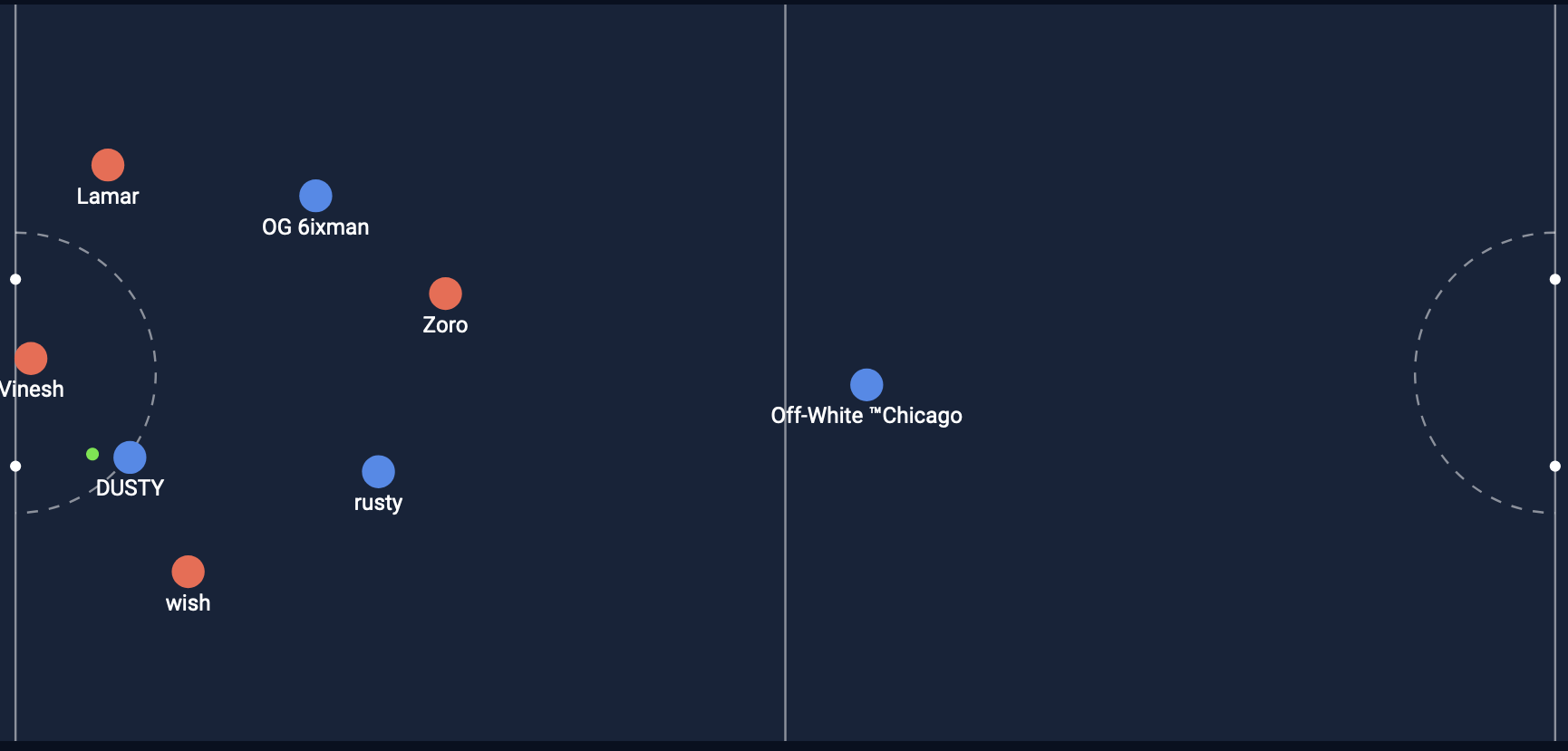
Shot #1
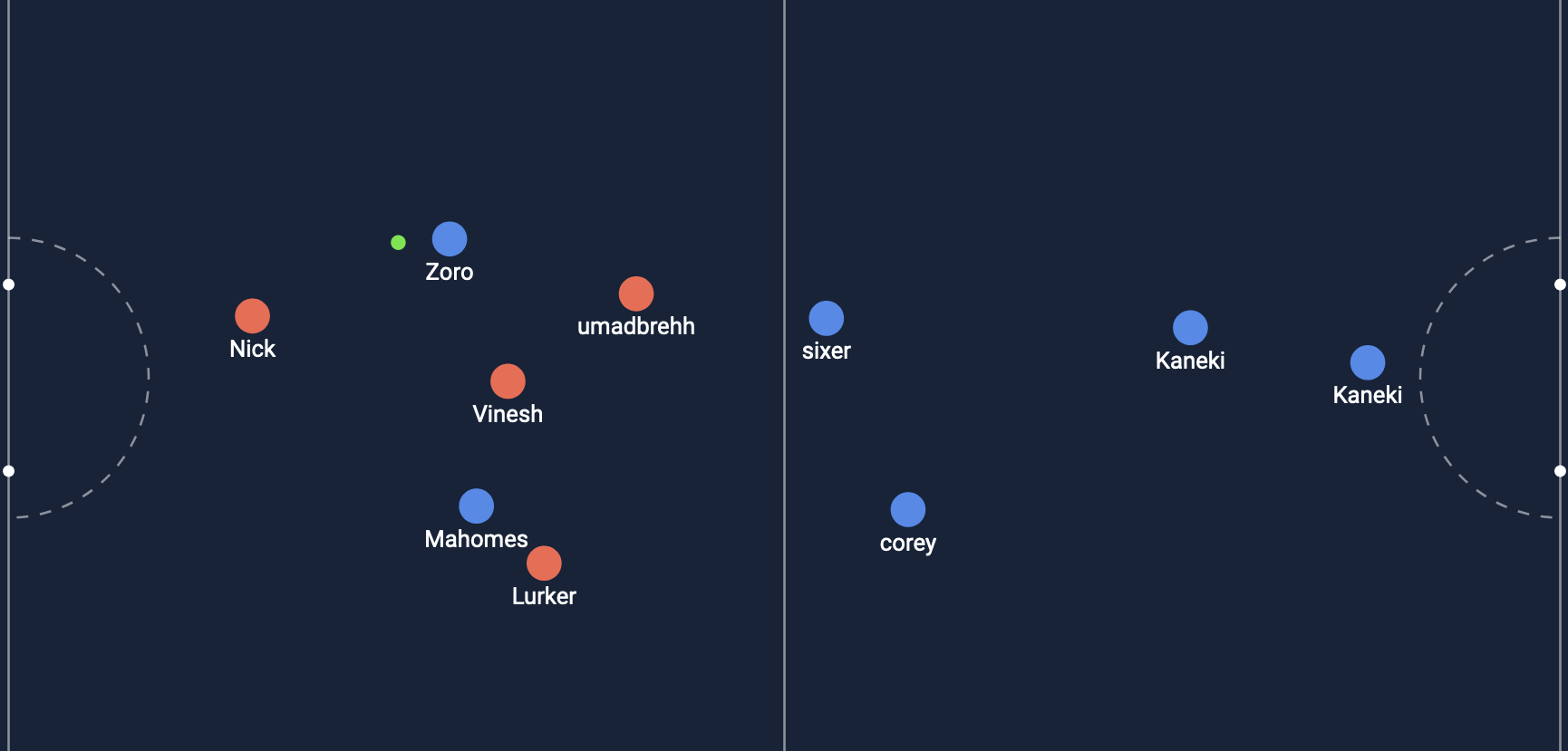
Shot #2
From the two pictures shown above, which shot is more likely to be a goal in your opinion?
- Shot #1
- Shot #2
Now lets look at the expected goal score that my model predicted…
Shot #1
Expected Goal = 0.193
Shot #2
Expected Goal = 0.510
Note: If you are not sure what these values mean, don’t worry! I will explain it soon.
Now with the images and the expected goal value, which shot is more likely to be a goal in your opinion?
- Shot #1
- Shot #2
Let’s dive deeper into this project and see what the expected goal (XG) is and how I was able to make a machine learning model predict it!
Let’s look at the replay!
Shot #1
Shot #2
The second shot was actually the one that went in! My model was able to predict a higher XG for the goal that went in. Let’s look at how the model works!
What is Haxball?
The gameplay shown in the animations above was taken directly from HaxBall. HaxBall is a 2D physics-based online multiplayer soccer game. Each user is a circle and can interact with the game using the arrow keys to move and the space bar to pass or shoot. HaxBall supports many kinds of matches, I trained my models on 3v3 and 4v4 matches.
What is XG?
Expected Goals or XG is a numerical value that estimates the probability of a kick to score. XG can also be calculated for specific players, kicks, or entire teams.
An XG of one means that a kick will 100% go into the goal and an XG of 0.5 means that it has a 50% chance of going in. XG can take into account multiple factors such as distance from the goal, defender positions, goal angle, and many other factors as well!
We design XG to gain insight about a team’s overall performance and shot quality, it can never be 100% correct and accurately predict all goals since soccer is far too complicated.
This video summarizes XG and what you need to know about it:
Why not just use shots on goal instead of XG?
Many of us are used to hearing about shots on goal as the main statistic that pops up on the screen while watching soccer. So you may be wondering why we need XG when we have shots on goal.
Shots on goal doesn’t take into consideration anything other than the number of shots a team had. Whether the shot was from the midline or a shot within the box, you still get one more shot added onto the shots on goal. XG takes into account the quality.
Here is a video that contains more information about the differences:
Haxball Machine Learning Project!
HaxBall is a popular game with its own API and Vinesh created a way to collect a large dataset from the game. Edwin and I were the first two people to work on this HaxBall dataset! This unique project had multiple steps to it. The first was to explore the data, then brainstorm and develop features for the models, and finally compare different models and deploy them!
What data was collected?
Each match record contains these seven kinds of data. Here are all seven kinds with some examples of what is stored in them. You can find the complete data schema in the HaxClass repo.
- score: One record that describes the final score.
- red: Number of goals scored for the red team.
- blue: Number of goals scored for the blue team.
- time: Duration of the match, in seconds, including overtime.
- scoreLimit: Number of goals needed to win by goals.
- timeLimit: Time limit in seconds for regulation.
- stadium: One record that describes the stadium name which is mapped to additional data in a dictionary
- Ex: “NAFL Official Map v1”
- goalposts: The coordinates and size off all four posts
- bounds: The field X and Y coordinates for bounds
- ball: Radius of the ball
- players: List of players in the game
- id: Numerical ID for player, unique for the match, but may not be the same across matches.
- name: Player screen name.
- team: Player team at the end of the match, either red or blue.
- goals: List of the goals scored
- kicks: Lists of times players kicked the ball
- possessions: Lists of periods when players possessed the ball
- start: Match time when the possession started, in seconds.
- end: Match time when the possession ended, in seconds.
- playerId: Numerical ID of player who possessed the ball.
- playerName: Screen name of player who possessed the ball.
- team: Team of player who possessed the ball
- positions: Lists of the positions of players at each time step.
When I started this project, I had to work with the codebase and dataset that Vinesh had created. This meant I had to take time to understand the data schema and code and how to work with it before being able to improve on it. This dataset that we had was large and it was in a challenging format. There were thousands of different matches with millions of data points about player positions and shots.
I took time to delve into the data and analyze it and test my knowledge by writing small code to try to obtain the data I wanted. Once I finished that, I was able to brainstorm multiple features I wanted to start developing in order to improve on the model!
Which features were created?
Before I started developing the features of the project, I was able to get feedback from students who played a few HaxBall games and look at Edwin’s model predictions. This feedback helped me understand a user’s point of view and helped me brainstorm further about how to improve the model based on that feedback.
My features that I wanted to create were:
- Player Speed: Speed of the players when the shot occured
- Zone separation: Separate the field into zones
- Shot intersection: Based on the angle of the player to the ball, check if path intersect between the goalposts
- Weighted post hits: Award 0.5 for hitting the post or being close to the goal
- Weighted defenders: Apply weights to defenders based on how close they are to the goal or the player who is shooting
I was able to develop the player speed feature, add on to Edwin’s code for the weighted defender feature, and create the shot intersection feature, which was the most complicated. Let’s take a closer look at my features.
Shot intersect
Here is the pseudo code for the feature:
- Find the frames for just the shooter and the ball
- Look backwards through the frames
- Find the frame that has a distance that is <= 30
- Once found, make that the frame to compute the intersection
 - If not found, get the last frame before the ball was kicked. When the distance between the ball and player starts increasing, we know the ball was kicked
- Get the goalpost positions
- Get the y-value of the ball when the x-value is equal to goalpost using point-slope
- Check if the y-value is in between the goal posts
- Return 1 if shot is on goal, .5 if it hits the post, and 0 if it isn't on goal
You can find the full code here
I was able to draw the intersections calculated by my feature to ensure I was computing it correctly. This is a sample from one shot:
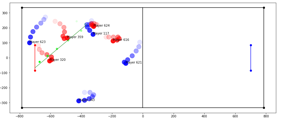
The green line is what the feature predicts the path of the ball and intersection will be and the green circles were the actual path from the match. My feature is able to predict it well but it is not exact since we had to search for the frame closest to when the player kicks the ball because we don’t know exactly when they do, so a small difference in position can lead to possibly a large angle change in course.
Player speed
Pseudo code:
- Get a time range to be able to measure distance
 - Start time is kicktime minus an offset
- Get the first and last position of a player from the start time till the ball was kicked
- Return the distance between the two positions divided by the time
Player speed can have a big effect on the shot and this feature greatly impacted precision. With Edwin’s feature for ball speed and this player speed feature, we were able to greatly improve the model predictions.
Weighted Defender Distance
Pseudo code:
- Get the closest defender to the shooter
- Count the number of defenders within a radius
- If a defender is closer than 4 units, then add .5 to the weight of the defender
This small enhancement was able to improve the model and surprisingly, some models improved when I had both the weighted defender distance I created and the similar feature Edwin created.
What models were tested and used?
There are many different algorithms out there for machine learning! This article compares some of the most popular ones and goes into some of the math of them if you are interested in that.
I tested the following models:
- K-nearest neighbors
- Decision Trees
- Random Forest
- Ada Boost
- GaussianNB
I noticed that Random Forest consistently ranked higher in all metrics so I decided to stick with that. Random Forest uses ensemble learning which combines learning models in order to increase the overall result. It has the ability to build many decision trees and then merges them in order to get more accuracy and better predictions.
Overall results and improvements
For this project, our main focuses were on these metrics of the model:
- Accuracy
- Precision
- Recall
- Area under the ROC curve
Accuracy is the number of correctly predicted data points out of all the data points. Precision answers what proportion of positives identifications was actually correct Recall answers what proportion of true positives was identified correctly? Area under the ROC curve tells you how good your model is at ranking predictions
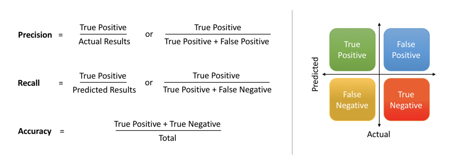
Image gotten from this article
Note: A true positive is when the model correctly predicts a scored goal. True negative when it correctly predicts a missed goal. False positive is when the model incorrectly predicts that a miss will score. And false negative is when the model incorrectly predicts that a goal will miss.
When we build a model,we need to choose a train/test split. We use this split because it allows us to fit the model on a training set and then see the predictions on the test data that wasn’t trained. The results allow us to compare the performance of the model for the predictive XG problem.
The results below are from the testing data since those are the important metrics that help us evaluate the performance of the model.
These were Edwin’s final results:
| Model | Features | Accuracy | Precision | Recall | ROC AUC |
|---|---|---|---|---|---|
| Random Forest (max_depth=12) | goal_distance, goal_angle, defender_dist, closest_defender, defenders_within_box, in_box, in_shot, ball_speed | 0.978 | 0.729 | 0.197 | 0.598 |
Note: Edwin’s results here are slightly different from his blog post because after Edwin deployed his models, we changed the filtering to only 3v3 and 4v4 match stadiums. These are the performance scores for Edwin’s model on the same test dataset as mine so that we can make sure to compare more accurately.
These are my results of my top two models after improving:
| Model | Features | Accuracy | Precision | Recall | ROC AUC |
|---|---|---|---|---|---|
| Random Forest (max_depth=15) | goal_distance, goal_angle, defender_dist, closest_defender, defenders_within_box, in_box, in_shot, ball_speed | 0.980 | 0.745 | 0.320 | 0.658 |
| Random Forest (max_depth=15) | goal_angle, goal_distance, defender_dist, closest_defender, in_box, defenders_within_shot, in_shot, ball_speed, on_goal, player_speed, weighted_def_dist | 0.980 | 0.767 | 0.292 | 0.645 |
Both of these models are deployed but I decided the to compare the first one since my main goal was to improve recall
My improvements were:
| Accuracy | Precision | Recall | ROC AUC |
|---|---|---|---|
| Before: 0.978 | Before: 0.729 | Before: 0.197 | Before: 0.598 |
| After: 0.980 | After: 0.745 | After: 0.320 | After: 0.658 |
| Improvement: (+0.2%) | Improvement: (+1.6%) | Improvement: (+12.3%) | Improvement: (+.06%) |
The project started out with a very poorly-performing model and Edwin had the challenge of producing much stronger models. My challenge was to continue improving a strong model, which brings up the challenge of “long tail”.
This is the statistical long tail curve:
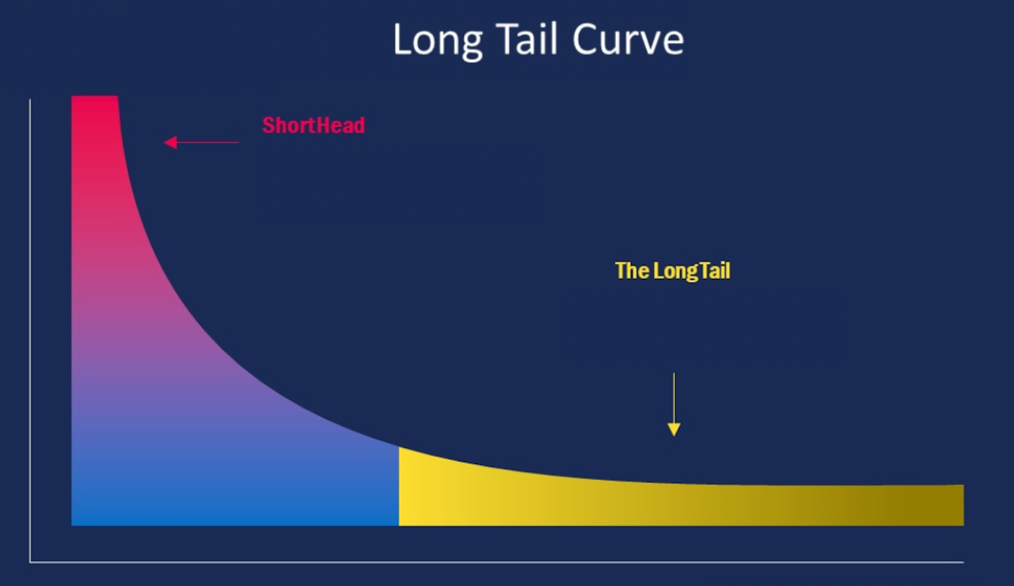
Image gotten from here
This model has learned to predict XG for some common goals, but the long tail is filled with many kinds of goals that might be less common or unexpected in some way. Making progress on predicting those goals will be slower and more incremental than the short head.
It was difficult trying to get the remaining 28% precision and 83% recall that was needed to get 100% in both categories. However, there is a ceiling of how good our model can really get. Just like in real life soccer, in Haxball there could be shots that were highly unlikely that go in and shots that are very easy that don’t go in. I was tackling “long tail” because I started off with a strong model as my benchmark so improving on a strong model by a little bit can be compared to improving a weak model by a lot.
The hardest part of trying to get this improvement is the precision recall tradeoff. If you increase the precision, then recall will decrease and vice versa. I was able to get one model to get to 90% precision but the recall dropped drastically. I wanted to focus on increasing recall while not letting the precision drop.
I used ablation testing, which is a way to understand the contribution and impact of a certain component by removing it in one model and comparing it to another model that has it. I was able to see that my features and models specifically were able to increase precision by 1.6% and recall by 12.3%!
What were the main takeaways from the project?
This unique project was a great opportunity for me to learn about many different aspects of software development and machine learning!
Building on top of someone else’s code
Most class projects make you start coding from scratch or give you very minimal starter code that is fairly easy to understand. However, in the real world as a software developer and in this project, you have to build on top of old code. Writing code is very important, but understanding others’ code is a very important skill. This also means that when I write code, I will always try to put comments and make it as understandable as I can so that I can make the next person’s life a bit easier!
User feedback is very important
One of my most complicated features was the shot intersection feature. While I was in the meeting getting user feedback from Edwin’s model, one player pointed out that one goal was an “open goal” that was shot directly towards the goal and yet the predicted XG was low. This gave me the idea to get where the shot should intersect in order to better predict if it will go in. Thanks to the user feedback, I was able to create a cool feature that improved the model!
Understanding data schemas make life easier
I never had to understand data that is this large and complicated. The dataset is unique and the format can get confusing. I learned that before developing any feature, I had to know the data very well or else I would be wasting time debugging data structure related errors.
Keep scaling in mind at the start of any project
I had the ability to work on a scaling problem in this project as well. Once my model was deployed, Vinesh noticed that the loading time for the models drastically increased. We wanted to make sure that as more models are deployed, this problem doesn’t occur. I was able to get the models to be lazily evaluated instead of loading all the models at once. This means that only the default model will be loaded right away but all the other models will only be loaded when the user wants to see their predictions. Before this improvement, it took 7.3 seconds to start up the server and after it went all the way down to 2.5 seconds!
How to view my model?
My model has been deployed and is live for you to check out!! You can also see the Haxml repo to view my contribution.
Haxml repo with my contributions on github
My model predictions on real matches in Haxball
My model predictions on the latest HaxBall matches
Contact Information
Email: lmatar@hawk.iit.edu
Special Thank you to…
Vinesh Kannan for getting all this data and giving me the opportunity to work on the project and learn so much!